Styling lines and markers with Matplotlib
Categories: matplotlib
In this article, we will learn how to apply styling to plots. This applies to line plots, scatter plots, and stem plots. Formattimg options include:
- Changing the colour, thickness, and dash style of the lines in a plot.
- Changing the colour, shape, and other attributes of the markers in a plot. Markers are the dots on a scatter plot or stem plot, but they can also be added to a line plot.
There are two ways to do this. We can use format strings, which are very simple to add but have a limited number of options. Or we can use formatting parameters, which have a lot more flexibility. We will look at both methods here, but first we will look at the default styling.
The code examples in this article are here on github, in the files linestyles.py and markerstyles.py.
Default styling
All the examples in this course so far have used default styling. This uses thin blue lines for the graph lines and small blue dots for the markers.
When we plot two data sets, the second one is automatically coloured orange to distinguish it.
This is useful for quick plots, but there may be situations where we want more control over the styles.
Styling lines using format strings
We can set the colour and line style for a graph by adding an extra string parameter to the plot function:
import matplotlib.pyplot as plt

x = [n/4 for n in range(20)]
y1 = [n*n for n in x]
y2 = [25 - n*n for n in x]

plt.plot(x, y1, "m")
plt.plot(x, y2, "-.r")
plt.show()
Here is the resulting graph:
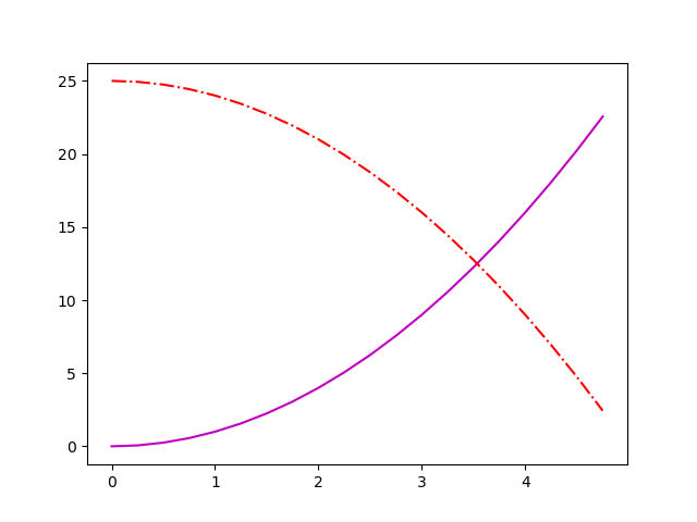
We are using artificial data for these plots, created using list comprehensions. The details don't matter too much, but we create a list x with 25 elements that count up from zero in steps of 0.25. We then create two lists, y1 and y2 that contain simple functions of x as an example plot.
When we plot the two graphs, we add an extra string parameter:
plt.plot(x, y1, "m")
plt.plot(x, y2, "-.r")
For the first plot, "m" sets the colour of the line to magenta.
For the second plot "-.r" sets the style to dash-dot, and the colour to red.
Format string options
The format string consists of three optional parts:
[marker][line][colour]
The [marker] part specifies the shape of the markers (see later). Options are:
- . (full stop character) gives a small circle or "point" marker
- , (comma character) gives a single pixel marker
- letter o gives a circle, larger that the point marker
- letter v gives a triangle, pointing down
- ^ (hat character) gives a triangle pointing up
- < (less than character) gives a triangle pointing left
- > (greater than character) gives a triangle pointing right
- number 1 tri down (tri is a 3 pointed "star" shape)
- number 2 tri up
- number 3 tri left
- number 4 tri right
- letter s square
- letter p pentagon
- * (asterisk character) star
- letter h hexagon1 (points up/down)
- letter H hexagon2 (points left/right)
- + (plus character) plus
- letter x cross
- letter D diamond
- letter d thin diamond
- | (pipe character) vertical line
- _ (underline character) horizontal line
The [line] part specifies the line style:
- - (single hyphen character) solid line
- -- (two hyphen characters) dashed line
- -. (a hyphen and a full stop) dash-dot line
- : (colon character) dotted line
The [colour] part specifies the colour of the line and/or markers:
- b blue
- g green
- r red
- c cyan
- m magenta
- y yellow
- k black
- w white
So in the previous example:
- "m" represents the colour magenta. There is no marker or line element.
- "-.r" represents the line style dash-dot ("-.") and the colour red ("r"). There is no marker.
Styling lines using parameters
As an alternative, we can set the colour and line style for a graph using named parameters of the plot function. Named parameters give us more options for each aspect of the appearance:
plt.plot(x, y1, color="cadetblue", linewidth=4)
plt.plot(x, y2, color="#ff8000", linewidth=6,
         linestyle=(0, (4, 2, 1, 2)), dash_capstyle="round")
plt.show()
Here is the resulting graph:
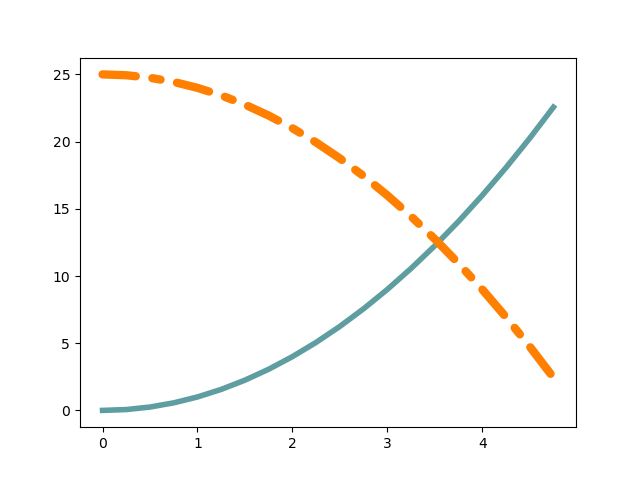
The data is created in the same way as before, so we haven't duplicated the code.
For the first plot, we supply these parameters:
color="cadetblue"sets the colour to a CSS named colour (in this case a blue-green colour). There are other options, see below.linewidth=4sets the line thickness to 4 pixels.
For the second plot, we supply these parameters:
color="#ff8000"sets the colour to hex value ff8000 (orange), see below.linewidth=6sets the line thickness to 6 pixels.linestyle=(0, (4, 2, 1, 2))sets the dash pattern, see below.dash_capstyle="round"- this causes each dash to have rounded ends (rather than the default square ends).
Line width
The line width of a Matplotlib plot is controlled by the linewidth parameter. You can also use the lw parameter - it does exactly the same thing, but it is a shorter name.
The line width is measured in points, where one point is one seventy-second of an inch (ie there are 72 points in an inch). Since the default resolution for a graph image created by Matplotlib is 100 pixels per inch this means that the linewidth parameter of a plot is approximately equal to the line width in pixels.
Colour specifiers
Colours are defined by a string value, but there are various ways to do this. Here are the main ones:
- A single letter (such as "b" for blue) specifies one of the 8 colours in the previous list.
- A name (such as "cadetblue") specifies one of the CSS named colours. There are 140 named colours, you can find a list of them online.
- A six-digit hex code (such as "#ff8000") specifies the RGB components as hex values, for example 0xff red, 0x80 green, 0x00 blue.
Line style specifiers
The linestyle is specified by a tuple of the form:
(offset, (on, off, on, off ...))
offset is normally zero, but can be used to shift the start point of the dash pattern.
(on, off, on, off ...) specifies the dash and gap lengths. So for example (4, 2, 1, 2) specifies a dash of length 4, a gap of 2, a dash of 1, and a gap of 2. This pattern is then repeated. Lengths are specified as multiples of the line width. So with a line width of 6, a dash length of 4 would be 24 pixels long.
The on-off list must have an even number of entries so that every "on" is followed by an "off".
Styling markers using format strings
We can add markers to the plot by adding a marker component into the format string:
plt.plot(x, y1, "sk")
plt.plot(x, y2, "^:c")
plt.show()
Here is the resulting graph:

This adds a small shape for every data point. For example:
- "sk" represents the marker style square ("s") and the colour black ("k"). There is no line style. This plots black squares with no line, similar to a scatter graph.
- "^:c" represents the marker style triangle ("^"), line style dotted(":"), and the colour cyan ("x"). This plots a cyan dotted line and also marks the points with cyan triangles.
Styling markers using parameters
We can add markers to the plot by adding parameters:
plt.plot(x, y1, color="#00ff40", linewidth=2, marker="h",
         markersize=8, markeredgecolor="indigo",
         markeredgewidth=2)
plt.plot(x, y2, color="goldenrod", linewidth=4, marker="D",
         markersize=10, markerfacecolor="midnightblue",
         markeredgewidth=2, markevery=4)
plt.show()
Here is the resulting graph:

For the first plot, we supply these parameters:
color="00ff40"sets the colour to light green.linewidth=2sets the line thickness to 2 pixels.marker="h"sets the marker shape to hexagon.markersize=8sets the size of the marker to 8 pixels.markeredgecolor="indigo"sets the colour of the outline of the marker to indigo.markeredgewidth=2sets the line width of the outline of the marker to 2 pixels.
This draws a green line with hexagonal markers. The markers are outlined in indigo, but the inside of the markers is green (like the lines) because we didn't specify any other colour.
For the second plot, we supply these parameters:
color="goldenrod"sets the colour to gold.linewidth=4sets the line thickness to 2 pixels.marker="D"sets the marker shape to diamond.markersize=10sets the size of the marker to 10 pixels.markerfacecolor="midnightblue"sets the colour of the inside of the marker to dark blue.markeredgewidth=2sets the line width of the outline of the marker to 2 pixels.markevery=4only draw a marker for every 4th data point,
This draws a gold line with diamond markers for data points 0, 3, 7 etc. The markers are filled with dark blue, but the outline of the markers is gold (like the lines) because we didn't specify any other colour.
Summary
We have seen how to control the line colour and style of line plots, and also how to add markers to the data points.
These same techniques can be used with other plots, for example stem plots or scatter graphs.
Related articles
Join the GraphicMaths/PythonInformer Newsletter
Sign up using this form to receive an email when new content is added to the graphpicmaths or pythoninformer websites:
Popular tags
2d arrays abstract data type and angle animation arc array arrays bar chart bar style behavioural pattern bezier curve built-in function callable object chain circle classes close closure cmyk colour combinations comparison operator context context manager conversion count creational pattern data science data types decorator design pattern device space dictionary drawing duck typing efficiency ellipse else encryption enumerate fill filter for loop formula function function composition function plot functools game development generativepy tutorial generator geometry gif global variable greyscale higher order function hsl html image image processing imagesurface immutable object in operator index inner function input installing integer iter iterable iterator itertools join l system lambda function latex len lerp line line plot line style linear gradient linspace list list comprehension logical operator lru_cache magic method mandelbrot mandelbrot set map marker style matplotlib monad mutability named parameter numeric python numpy object open operator optimisation optional parameter or pandas path pattern permutations pie chart pil pillow polygon pong positional parameter print product programming paradigms programming techniques pure function python standard library range recipes rectangle recursion regular polygon repeat rgb rotation roundrect scaling scatter plot scipy sector segment sequence setup shape singleton slicing sound spirograph sprite square str stream string stroke structural pattern symmetric encryption template tex text tinkerbell fractal transform translation transparency triangle truthy value tuple turtle unpacking user space vectorisation webserver website while loop zip zip_longest