Advanced vectorisation in numpy

NumPy vectorisation applies a function to an entire array in one call. For example:

a = np.array([1, 2, 3])
b = np.array([4, 5, 6])
u = np.sqrt(a)  # [1. 1.414 1.732]
v = a + b       # [5 7 9]

Calling np.sqrt calculates the square root of every element in a. Using the + operator results in the np.add function being called, performing elementwise addition of the 2 arrays.

These operations are very efficient, because the looping is done in optimised C code. This is called vectorisation.

But NumPy also allows you to so more advanced types of vectorisation, which we will look at in this article.

Fancy indexing

Fancy indexing allows you to use one array as an index into another array. It can be used to pick values from an array, and also to implement table lookup algorithms.

Here is a simple example:

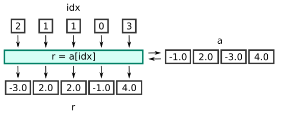
a = np.array([-1.0, 2.0, -3.0, 4.0])
idx = np.array([2, 1, 1, 0, 3])
r = a[idx]

Here the array a is the array of source values.

The array idx contains integers that act as indexes into the array a. So, for example, the value 2 in idx indexes element 2 in a (which has the value -3.0), etc. While the source array a can use any data type (it is a float array in the example), the idx array must be an integer type.

Now look at the final line:

r = a[idx]

Normally a[n] fetches the nth element from a. But because we are passing in an array, idx, the statement fetches an array of elements.

idx has values 2, 1, 1, 0, 3. If we look at r it contains:

[-3.  2.  2. -1.  4.]

The array has been filled with element 2 from a (which is -3.0), then element 1 from a (which is 2.0), then element 1 again, and so on.

This is called fancy indexing. It selects values from a based on the index values in idx.

Notice that the length of r is the same as the length of idx, rather than a. This diagram illustrates the process:

Here is the equivalent code using a loop:

a = np.array([-1.0, 2.0, -3.0, 4.0])
idx = np.array([2, 1, 1, 0, 3])
r = np.empty_like(idx, dtype=a.dtype)
for i in range(idx.size):
    r[i] = a[idx[i]]

The fancy indexing version is generally far more efficient than the loop.

Fancy indexing with multidimensional index

We can use fancy indexing with a multidimensional index array, like this:

a = np.array([-1.0, 2.0, -3.0, 4.0])
idx = np.array([[2, 0, 1], [3, 3, 0]])
r = a[idx]

This works in the same way as before, each value in the idx array is used to select a value from the a array.

The result is an array with the same shape as idx:

[[-3. -1.  2.]
 [ 4.  4. -1.]]

Fancy indexing with a boolean index

The previous description applies for index arrays of type integer. We can also use a boolean index array, which behaves slightly differently.

a = np.array([-1.0, 2.0, -3.0, 4.0])
idx = np.array([True, False, False, True])
r = a[idx]

The output array r contains the values from a where the corresponding element in idx is True.

In this case, elements 0 and 3 of idx are True, so elements 0 and 3 of a are selected. The result, stored in r, is the array:

[-1.  4.]

The rules for this case are slightly different to thr previous examples:

• a can be of any type.
• idx must be of Boolean type.
• The shape of idx must exactly match the shape of a.
• The length of the output array will be determined by the number of True values in a.

The where parameter

All universal functions have a where parameter.

The where parameter takes an array of booleans. It applies the function only where the array is true. For example:

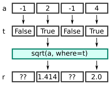
a = np.array([-1.0, 2.0, -3.0, 4.0])
t = a>0
r = np.sqrt(a, where=t)

Here we first create an array t that is true wherever the value in a is greater than 0. That is:

t = [False  True False  True]

When we calculate the square root, the calculation is only performed where t is true, so we don't attempt to calculate negative square roots. This means that in the output array b, values are only calculates for elements 1 and 3:

r = [?? 1.41421356 ?? 2.]

Elements 0 and 2 of r are left unchanged (shown as ??). If you run this example yourself, r starts off as an empty array, so elements 0 and 2 are uninitialised. They will just contain whatever happened to be in memory.

You can visualise it like this:

Here is the equivalent code using a loop:

a = np.array([-1, 2, -3, 4])
t = a>0
b = np.empty_like(a)
for i in range(a.size):
    if i[i]:
        b[i] = sqrt(a[i])

Using the where parameter allows us to perform the same functionality as the loop, but with the speed of a vectorised function.

We can control the content of the unassigned elements by initialising the output array to a particular value (for example using full_like), and then use out to update that array:

a = np.array([-1.0, 2.0, -3.0, 4.0])
r= np.full_like(a, -1.0)
np.sqrt(a, where=a>0, out=r)

This initialises r to -1.0, so that any elements that are left unchanged by where will remain set to -1.0:

r = [-1.          1.41421356 -1.          2.        ]

The at function

The at function does something similar, but uses an index array to control which elements are calculated.

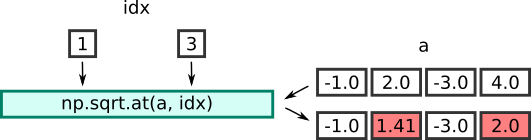
a = np.array([-1.0, 2.0, -3.0, 4.0])
idx = [1, 3]
np.sqrt.at(a, idx)

In this case we are using the usual value for a, and index array idx indicates that only elements 1 and 3 should be calculated. The at function updates these elements in place - it modifies these elements of the array a, leaving the other elements unchanged. Here is the result:

a = [1.          1.41421356 3.          2.        ]

One interesting thing to note here is that at isn't a parameter of the sqrt function, it is a method of the sqrt function. In Python, functions are objects, and objects can have methods, so a function can have methods.

Here is an illustration of the process:

Summary

Universal functions are a very efficient way of performing an operation on every element of an array. NumPy also has extra ways to perform conditional processing on selected elements in an array.

See also

• Universal functions in in numpy
• Broadcasting in in numpy
• Reducing and accumulating numpy arrays