Bezier curves in Pycairo

This article describes how to draw Bezier curves in Pycairo.

What is a Bezier curve?

A Bezier curve is a versatile mathematical curve that can be used to create a wide variety of different shapes in vector graphics. The curve is controlled by 4 points, A, B, C and D:

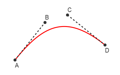
The curve starts at point A and ends at point D. These two end points are sometimes called the anchors. The shape of the curve is controlled by points B and C - these points are sometimes called the handles.

Here is how to draw a Bezier curve using Pycairo:

ctx.move_to(ax, ay)
ctx.curve_to(bx, by, cx, cy, dx, dy)

In the code, point A is represented by coordinates (ax, ay), point B by (bx, by) etc.

Here is how it works:

• move_to sets the current point to point A.
• curve_to draws a curve from the current point A to the point D, using B and C as handles.

Here is the full Python code to draw a Bezier curve:

import cairo

# Set up Pycairo
surface = cairo.ImageSurface(cairo.FORMAT_RGB24, 400, 250)
ctx = cairo.Context(surface)

# Paint the background
ctx.set_source_rgb(1, 1, 1)
ctx.paint()

# Draw the image
ctx.move_to(50, 200)
ctx.curve_to(150, 75, 225, 50, 350, 150)
ctx.set_source_rgb(1, 0, 0)
ctx.set_line_width(2)
ctx.stroke()

# Save the result
surface.write_to_png('bezier.png')

Bezier curve shapes

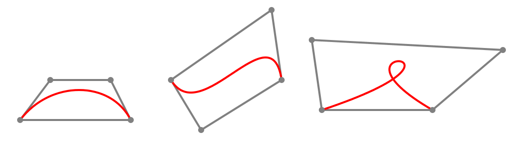
Depending on the positions of the handles relative to the anchors, a Bezier curve can create a variety of different shapes. Here are some examples:

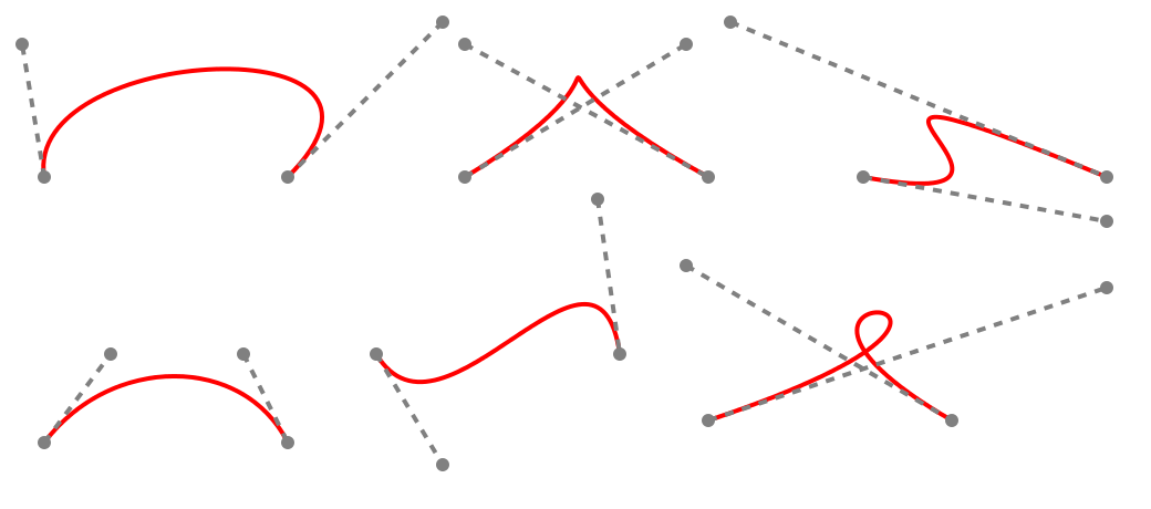
As you can see, this includes simple curves, S-shaped curves, curves with cusps, and even loops.

If you want to explore Bezier curves dynamically, you could use any drawing package that supports Bezier curves. All the curves shown have the similar anchor points, the different shapes are created by moving the handles as shown.

Bezier curve extents

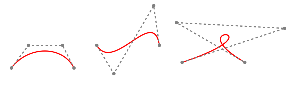
The control polygon is formed joining the control points in the strict order A, B, C, D. This can form either a simple quadrilateral, an S shape, or a self-intersecting X shape.

The general shape of the Bezier curve will follow the form of the control polygon, as in these examples:

You can also form a convex hull of the points A, B, C, D. The convex hull is the smallest convex polygon that encloses all 4 points. The Bezier curve will always be entirely contained within the convex hull:

Joining Bezier curves

It is quite easy to join two or more Bezier curves. We just need to define the curves so that they have a shared anchor point.

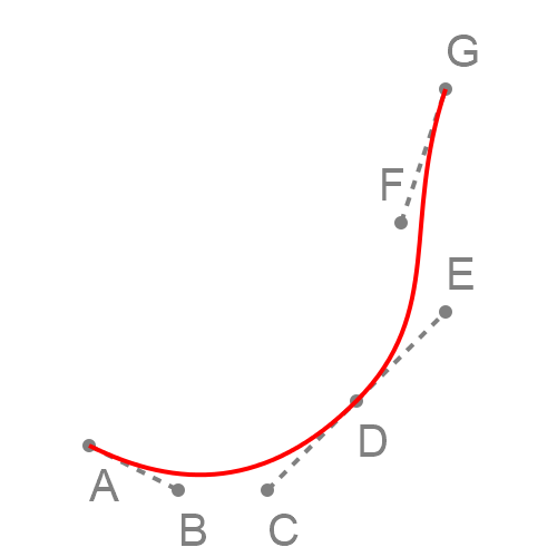
The diagram below shows two Bezier curves that are joined. The first curve has anchor points A and D, with handles B and C.

The second curve has anchor points D and G, with handles E and F. Since the curves both have point D as an anchor, they are joined at that point.

The code to draw two joined Beziers looks like this:

ctx.move_to(ax, ay)
ctx.curve_to(bx, by, cx, cy, dx, dy)
ctx.curve_to(ex, ey, fx, fy, gx, gy)

Here is how it works:

• move_to sets the current point to point A.
• curve_to draws a curve from the current point A to the point D, using B and C as handles.
• After executing curve_to the current point is set to D
• The second curve_to draws a curve from the current point D to the point G, using E and F as handles.

Smooth curves

In the diagram above, you will notice that the two Bezier curves form a corner where they connect. There is nothing wrong with that, it is sometimes what you want to create a particular shape.

Sometimes you might want two Bezier curves to join more smoothly, so it looks like a single curve, as shown below:

It is fairly easy to do this. The slope of a Bezier curve at its end point is equal to the slope of the line from the handle. That is:

• For the first curve, the slope of the curve at point D is the same as the slope of the line between C and D.
• For the second curve, the slope of the curve at point D is the same as the slope of the line between D and E.

This means that if the points C, D and E are all in a straight line (as they are in the example), the two curves will have the same slope where they meet, which avoids a corner.

In other words, to obtain a smooth join, make sure the handles of the two curves line up.

Another thing to know is that the second derivative of the curve at its end point is determined by the length of the line to the handle. The second derivative means the rate of change of the slope, or very loosely speaking how curved the Bezier curve is near its end point. If the two curves have the same slope and curvature, the join will be even more smooth.

In other words, to get the smoothest result when joining two curves, ensure that the handles C and E, and the anchor D are in a straight line, and also that C and E are both the same distance from D.

See also

• Drawing shapes in Pycairo
• Paths and complex shapes in Pycairo