Paths and complex shapes in Pycairo

Paths

A path is the most general type of shape. It is made up of one or more edges, than can consist of straight lines, arcs, or curves (specifically Bezier curves).

For example:

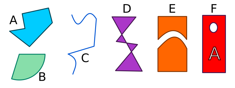
• Path A is created from 6 straight lines.
• Path B consists of 2 straight lines and a circular arc.
• Path C consists of 2 straight lines and 2 Bezier curves.

Each of the paths in the image has its own characteristics, to illustrate the variety of different forms a path can take:

• A and B are simple closed paths, that each enclose a single area. A is a polygon, B is a sector of a circle.
• C is an open path, it is just a set of lines that don’t enclose an area. An open path has two end points that are not joined together.
• D is a self-intersecting path. It is a polygon just like A, but some of its sides cross over, so it encloses several different areas (4 triangular areas in this case).
• E is a disjointed path. It consists of 2 separate closed shapes (each shape is actually a sub-path, which we will explain in the next section).
• F is also a disjointed path, this time consisting of 3 separate closed shapes, but this time the two small shapes (the ellipse and the letter A) actually cut holes in the main rectangular shape. If you placed this shape on top of an image background, you would be able to see the image through the holes.

As example F shows, paths can be text-shaped (the red shape has a text-shaped hole).

Paths are created implicitly, by calling drawing operations on the Pycairo context. But it is also possible to store the path you have created, as a Path object. This can be very useful sometimes as we will see.

Sub-paths

Any path is made up of one or more sub-paths. A sub-path is a set of lines or curves joined end to end – each line starts where the previous one ended. A sub-path therefore creates either a single closed shape, or a single set of sequentially joined lines.

In the picture above, each of the four shapes on the left is an example of a path containing a single sub-path. The two shapes on the right are each examples of single paths that are made up of more than one sub-path:

• The orange shape labelled E is made up of two sub-paths (each of the two closed shapes is a separate sub-path).
• The red shape labelled F is made up of three sub-paths (the rectangle itself is one sub-path, the circular hole is another, the A-shaped hole is another).

Letter shapes are a good, practical example of using sub-paths.

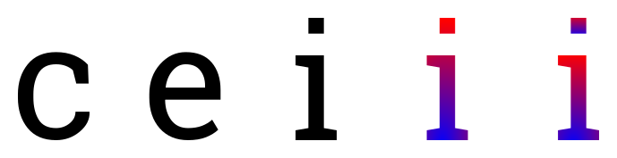
Each of these letters is drawn as a separate path. The letter 'c' is a simple closed path. The letter 'e' consists of a closed path but it also has a hole in it. This is formed as a sub-path, similar to the example of red shape F, above. Paths with holes aren’t just some fancy effect you might never use, the page you are reading contains hundreds of examples.

The letter 'i' is interesting. It consists of two separate shapes (the main character and the dot above it), but of course they are part of the same letter shape. You wouldn’t usually want to show one without the other, and you would always want them to be in the same position relative to each other – if you put the dot underneath the main character, for example, it wouldn’t be a letter 'i' any more! So it makes perfect sense to have those two shapes as two sub-paths of the same path.

The second letter 'i' shows another advantage of sub-paths. We have filled this letter with a gradient (the colour changes from blue to red, vertically). Since the two shapes are both sub-paths of the same path, the gradient is applied across the entire letter, from the base right to the top of the dot.

The third letter 'i' shows how the gradient might look if the two parts of the letter were drawn as completely separate paths. The dot now has its own blue to red gradient, which is probably not the effect you would want.

When we look at text in a later chapter, we will see that often a whole word (or sentence, or paragraph) of text is often drawn as a single path with lots of sub-paths (one or more for each letter).

Creating sub-paths

The most common way of creating a new sub-path is the move_to function. Here is some code that creates a path consisting of 3 sub-paths:

#Sub-path 1
ctx.move_to(50, 50)
ctx.line_to(400, 200)
ctx.line_to(50, 350)
ctx.close_path()

#Sub-path 2
ctx.move_to(450, 100)
ctx.line_to(550, 100)
ctx.line_to(450, 300)

#Sub-path 3
ctx.move_to(100, 100)
ctx.line_to(200, 200)
ctx.line_to(100, 300)
ctx.close_path()

ctx.set_source_rgb(1, 0, 0)
ctx.set_line_width(10)
ctx.stroke()

Sub-path 1 is started by the first move_to. It is a closed triangle with corners at (50, 50), (400, 200) and (50, 300). The call to close_path at the end of the definition closes the sub-path (ie it joins the final point to the initial point).

Sub-path 2 is started by the second move_to. It is an open shape with two sides. There is no close_path because the shape is not closed.

Sub-path 3 is started by the third move_to, and creates another closed triangle with corners at (100, 100), (200, 200) and (100, 300).

The final call to stroke draws the entire path (containing 3 sub-paths) and clears the path afterwards. Here is the image created:

You can also create a new sub-path using the context function new_sub_path. This is similar to move_to, but it doesn’t set the current point. It is mainly used with the arc function as described later in this chapter.

The final way to create a new sub-path is the rectangle function. This creates a closed rectangular sub-path.

Polygons

In this section we will look at a slightly more complex polygons – a useful arrow shape. This example will illustrate a few techniques than can be used generally to design polygons.

A simple arrow

Here we will see how to draw this arrow:

The size and position of the arrow is defined by its bounding box (x, y, width, height). The shape of the arrow can be adjusted by controlling the tail length a and inset b. The shape has 7 vertices, which we will number:

We can calculate the position of each vertex:

1. (x, y + b)
2. (x, y + height – b)
3. (x + a, y + height – b)

And so on. To draw the arrow, we just join the points to make a polygon. Here is a function that draws an arrow:

def arrow(ctx, x, y, width, height, a, b):
    ctx.move_to(x, y + b)
    ctx.line_to(x, y + height - b)
    ctx.line_to(x + a, y + height - b)
    ctx.line_to(x + a, y + height)
    ctx.line_to(x + width, y + height/2)
    ctx.line_to(x + a, y)
    ctx.line_to(x + a, y + b)
    ctx.close_path()

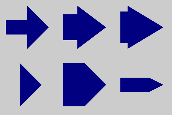
This code is quite versatile, we can create different arrow shapes by varying the size of the bounding box (width and height) and changing a and b. Here are some examples:

ctx.set_source_rgb(0, 0, 0.5)
arrow(ctx, 20, 20, 150, 150, 75, 50)
ctx.fill()
arrow(ctx, 220, 20, 150, 150, 50, 30)
ctx.fill()
arrow(ctx, 420, 20, 150, 150, 25, 20)
ctx.fill()
arrow(ctx, 70, 220, 75, 150, 0, 50)
ctx.fill()
arrow(ctx, 220, 220, 150, 150, 75, 0)
ctx.fill()
arrow(ctx, 420, 270, 150, 50, 100, 0)
ctx.fill()

This is the image the code creates:

Roundrect

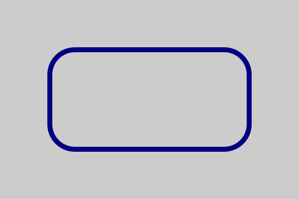
A roundrect is a rectangle with rounded corners:

It is defined by its position (x, y), width, height, and the radius r of the rounded corners. As the right-hand side of the diagram shows, a roundrect is made up of four quarter circles of radius r, with fours straight lines between them.

The most important points for drawing a roundrect are the centres of the corner circles. These are inset from the corners of the enclosing rectangle by an amount r. Starting from the top left corner and working clockwise, these centre points are:

• (x + r, y + r)
• (x+width-r, y+r)
• (x+width-r, y+height-r)
• (x+r, y+height-r)

The diagram below shows how we create the roundrect. The red solid lines show the arcs that we explicitly draw, the grey dashed lines show the connecting lines that Pycairo draws automatically:

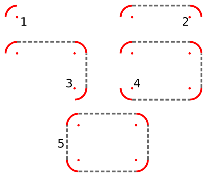
1. We draw the first quarter circle arc.
2. We draw the second quarter circle arc. Pycairo automatically draws a line from the end of the previous arc to start of the new arc.
3. We draw the third quarter circle arc, and again Pycairo draws a line from the end of the previous arc to the start of the new one.to start of the new arc.
4. We draw the fourth quarter circle arc, and again Pycairo draws the extra line.
5. Finally we close the path, so Pycairo adds a line from the end of the last arc to the start of the first arc, completing the shape.

Here is the code to do this:

def roundrect(ctx, x, y, width, height, r):
    ctx.arc(x+r, y+r, r, math.pi, 3*math.pi/2)
    ctx.arc(x+width-r, y+r, r, 3*math.pi/2, 0)
    ctx.arc(x+width-r, y+height-r, r, 0, math.pi/2)
    ctx.arc(x+r, y+height-r, r, math.pi/2, math.pi)
    ctx.close_path()

ctx.set_line_width(10)
ctx.set_source_rgb(0, 0, 0.5)
roundrect(ctx, 100, 100, 400, 200, 50)
ctx.stroke()

Here is the final result:

Function curves

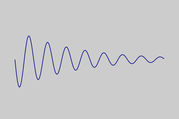
Sometimes you might want to draw a curve based on a mathematical function. Here is an example of a function y = f(x):

y = math.sin(10*x)*math.exp(-x/2)

This function is a decaying sine wave. It represents simple damped oscillation - for example, the sound created if you pluck a guitar string, that starts off loud and gradually fades away. Don't worry too much about the detail so of the function, we are mainly using it because it looks quite nice. This is a graph of the function created using Pycairo:

How is that done? Well, it is actually quite simple. We choose a series of value of x, and calculate f(x) for each value. This gives us a set of points that lie on the curve:

We then join this points with straight lines. In other words, we create a polyline from all the points.

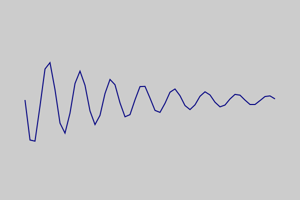
Now this looks pretty lumpy at the moment, you can clearly see the individual lines. That is deliberate, to show what is going on. The trick is to calculate more points that are closer together, then they look like a smooth curve.

D> This is actually very similar to what Pycairo does when it draws a Bezier curve or an arc. It splits the curve into a series of very small straight line segments, and draws those. This is called flattening the curve. It looks like a smooth curve but it is actually just straight lines.

Now we can move on to the actual code that creates the function curve above. Here is how we calculate the points:

x = 0
points = []
while x < 5:
    y = math.sin(10*x)*math.exp(-x/2)
    points.append((x*100 + 50, y*100 + 200))
    x += 0.01

The while loop iterates over values of x from 0.0 to (almost) 5.0 in steps of 0.01. The step value is very important, it determines the gap between the calculated points, which controls how smooth the curve is. You need to experiment a bit, if the gap is too big the curve won't be smooth, but if it is too small you will be calculating more points than you really need to.

For each x value, we calculate a y value using our function (the decaying sine wave function).

The result to of this is a set of (x, y) values that we want to plot. But there is a slight problem. Our x values are in the range 0.0 to 5.0. Our y values are in the range -1.0 to +1.0. If we plot those points on a canvas that is 600 units by 400 units, we will end up with a tiny graph stuck in the top corner!

We need to scale and translate our x and y values to create a set of points that have sensible canvas locations. Here is what we do:

• For x values we multiply by 100 and add 50. So x values in the range 0.0 to 5.0 create canvas values in the range 50 to 550 - ideal for a canvas that is 600 units wide.
• For y values we multiply by 100 and add 200. So y values in the range -1.0 to +1.0 create canvas values in the range 100 to 300 - also ideal for a canvas that is 400 units high.

We add these scaled points to the points list, as (x, y) tuples.

Plotting the points is now quite easy:

ctx.move_to(*points[0])
for p in points[1:]:
    ctx.line_to(*p)

ctx.set_line_width(2)
ctx.set_source_rgb(0, 0, 0.5)
ctx.stroke()

We move_to the location of points[0], and then call line_to on the rest of the points in the list to create a polyline. We then stroke the polyline.

See also

• Drawing shapes in Pycairo
• Bezier curves in Pycairo