Key advantages of NumPy

In this article, we will take a top-level look at the key advantages of using NumPy.

What is NumPy, and why do we use it?

At the heart of NumPy is the ndarray object. This is an array, a bit like a Python list, except that:

• It stores numbers as primitive data types.
• It is multidimensional.
• It has a fixed size.

A primitive data type just means that the data is stored directly as bytes. So for example, an image is usually composed of pixels, each with red, green and blue values between 0 and 255. In NumPy, each pixel is stored as three bytes, one per colour. The bytes of all the pixels are stored sequentially in memory. This is very compact and quick to access.

The NumPy library also includes lots of functions for manipulating ndarray objects. These make it very convenient to process arrays, but they are also very fast. They are written in C, a language that is very fast at processing arrays of primitive data types.

The fact that the data exists in memory as an array of primitive data types also means that the data can be easily be exchanged with other libraries that might be written in Python, C, or just about any other language there is.

These are the three basic advantages of NumPy - compact data storage, high-speed processing of arrays, and data compatibility with lots of other libraries. We will explore these further in the rest of the article.

1 Compact storage

We can create a Python list of numbers, like this:

k = [1, 2, 3, 4]

Here the list k is a Python object, and the 4 elements of that list are also Python int objects. A python int object will typically be around 28 bytes in size. The list itself will also need a pointer for each element, which typically adds another 8 bytes. The total data size will be 4 elements multiplied by (38 + 8) bytes per element, which is 144 bytes in total.

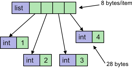
This is just the memory used to store the data. The list object itself also takes a small amount of memory, but we can ignore this when we consider large lists because it will be negligible compared to the per-element space.

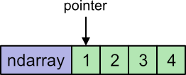
We can create a NumPy array like this:

data = np.array([1, 2, 3, 4], dtype=np.uint8)

The ndarray itself is a Python object. The array data is type np.uint8, which is 8-bit unsigned data. Each element takes 1 byte, so the array data is stored in memory as 4 bytes.

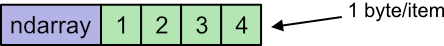
Again we will ignore the memory used to store the array object, it is small compared to the data for a large array.

Suppose we had a 24-megapixel image. Each pixel would consist of 3 byte values (red, green and blue) so there would be 72 M data values.

A NumPy array would store each value as a single byte, so the array would take 72 MByte of memory.

A Python list would store each value as a 28-byte object plus an 8-byte reference, so it would take over 2.5 GBytes of memory.

An application that had several large images open at the same time could save many GBytes of memory by using NumPy arrays, and that could make the difference between the application running smoothly or grinding to a halt.

2 Fast array loops

Consider two lists, and we wish to create a new list by adding the values together:

k1 = [0, 2, 4, 6, 8, 10]
k2 = [10, 20, 30, 40, 50, 60]
k3 = [x1 + x2 for x1, x2 in zip(k1, k2)] # [10, 22, 34, 46, 58, 70]

Here we have used a list comprehension, but we could have used a loop instead. Python uses an iterator to loop over a list. The iterator keeps track of where we are in the list. In addition, the list contains int objects, so to obtain the numerical value we must extract it from the object.

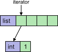
Python implements iterators and in objects fairly efficiently, but there are still several steps that need to be performed on every loop.

We can do a similar thing with NumPy arrays:

data1 = np.array([0, 2, 4, 6, 8, 10], dtype=np.uint8)
data2 = np.array([10, 20, 30, 40, 50, 60], dtype=np.uint8)
data3 = data1 + data2  # [10, 22, 34, 46, 58, 70]

Here we are using the + operator to add two arrays. ndarray overloads the + operator to perform an element by element addition of the two arrays (similar to the list case).

Aside from the much neater syntax, there is something else very important going on. The overloaded + operator accepts 2 arrays, and the task of looping over both arrays is performed internally, within the NumPy library. This is called vectorisation.

That loop is written in C. The code will typically use a memory pointer to keep track of where we are in the loop. A memory pointer is a primitive data type, so is very fast. In addition, the pointer will fetch a primitive integer directly from memory, which is a lot faster than extracting the value from an object.

In fact, in compiled C code it is usually possible to increment the pointer and fetch the value in a single instruction. It is a very fast operation.

NumPy also supplies special versions of the mathematical functions such as square root, sine, cosine. log etc that also run very quickly:

data4 = np.sqrt(data1)

These are called universal functions.

3 Slicing without copying

NumPy supports slicing, similar to Python lists. For example:

data5 = data1[1::2]  # [2, 6, 10]

This selects every second item from the array, starting at index 1. So it takes values 2, 6 and 10.

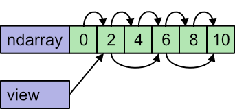
There is an important difference. When we slice a list we create a new list with the selected elements. But when we slice a NumPy array, we don't create a new array, We create a new view of the same data. When we access data1[0] it gets us the element 0 of the data. When we access data5[0], it gets us the element 0 of the data5 view of the data, which corresponds to element 1 of the underlying data set.

Also, if we loop over the original data1 the pointer starts at 0 and increments by 1 each time. But if we loop over the slice data5 the view knows that the pointer must start at 1 and increments by 2 each time:

For very large data sets, this amount to a high saving in execution time and memory, because we don't have to create a copy of all that data.

This does require a little care. If we were to modify the elements in data5, it would also affect data1, because it is the same data.

It is possible to force NumPy to create a copy of the data if you wish, using the copy method.

There are several other places that views are used, including the ones below:

Slicing of multidimensional arrays - a 2D array can be sliced either or both dimensions, selecting a rectangular region of the original array as a view. This can be done with more than 2 dimensions.

Transposing an array - for a 2D array this effectively flips the array about its leading diagonal. For higher dimensions, any combination of axes can be transposed. In all cases, a view is created.

Broadcasting - in broadcasting, NumPy automatically adds dimensions to an array to make it compatible for a calculation, as in this example:

a = np.array([[1, 2, 3],[4, 5, 6]])
b = np.array([10, 20, 30])
print(a+b)

Array a has 2 rows by 3 columns. Array b has (effectively) 1 row of 3 columns. You would not expect these arrays to be compatible for addition. However, broadcasting allows NumPy to automatically treat b as 2 rows of 3 columns, by repeating the first row. This is done using a view, that causes NukPy to read the same row twice. It doesn't require a 2 by 3 array to be created.

4 Array operations

NumPy supports many array level operations. These include:

• Joining and splitting arrays. For example, a 3D array representing a colour image (width by height by 3 channels for RGB) can be split into 3 separate greyscale images (width by height by 1). Or the 3 images can be joined.
• Arrays can be sorted and filtered.
• Reducing operators can be applied - for example finding the smallest value, or the sum of all the values.

5 Compatibility

Many Python libraries use NumPy internally. These include:

• SciPy.
• Pandas.
• Matplotlib.

ndarray, the basic NumPy array type, is used as a common data format for exchanging data between these different programs. And since an ndarray is just a multidimensional array of numbers, it can be used to represent anything - a computer image, a sound, a list of share prices, and so on.

Compatibility goes even further than this. The data within an ndarray can be stored in a memory buffer or file as raw data - just the data bytes. That format is not Python-specific, so the data can be exchanged with any program, written in any language, that understands basic binary data.

Pillow and Pycairo are two imaging libraries that can exchange data with NumPy in that way. They are both C libraries that have a Python binding. This method of exchanging data is universal and also quite efficient. It can be applied to almost any library that has a Python binding.

NumPy has various options for controlling low-level detail such as byte order, to allow compatibility with different memory models used by C and Fortran programs.

Summary

NumPy is a useful library with a wealth of functionality for dealing with arrays of numerical data. In addition, the implementation offers memory and execution efficiency that often comes close to compiled code, as well as serving as an interchange format for many existing libraries.

See also

• Anatomy of a numpy array
• Numpy efficiency